Can a convolutional neural network predict the stock market?

Partly. A 2023 Journal of Finance study found that a CNN trained on price-chart images predicted the direction of US stock returns better than classic momentum and reversal signals, out of sample from 2001 to 2019. The edge was strongest over the following week and in smaller stocks, and it shrank after trading costs.

Is a CNN or an LSTM better for stock prediction?

Neither wins by default. A CNN is good at short local patterns in a window of prices, while an LSTM carries a running memory through a sequence. The authors of the chart-image study say they cannot rule out that a well-built LSTM would beat their CNN, so test both on the same date-split data.

What is a probabilistic neural network?

A probabilistic neural network is a classifier that estimates how densely each class covers the space around a new example, using a kernel placed on every training point, and picks the most likely class. It trains almost instantly because it stores the data. It also slows down as the dataset grows, which limits it on long price histories.

Are LLMs neural networks?

Yes. A large language model is a neural network, usually a transformer, trained to predict the next token of text. It shares building blocks with the CNN in this article, such as learned weights and activations, at a far larger scale.

What is the delta in neural networks?

The delta is a neuron's error signal during backpropagation: the gradient of the loss with respect to that neuron's input before activation. Deltas are calculated at the output layer first and passed backwards to work out how much each weight should change.

How do you create a neural network for stock prediction?

Turn prices into returns and cut the series into fixed windows, each labelled with what happened next. Then train a small model such as the PyTorch CNN above, split by date with a gap between training and test data, and judge it on returns after costs.

Convolutional Neural Network Stock Market Models Explained

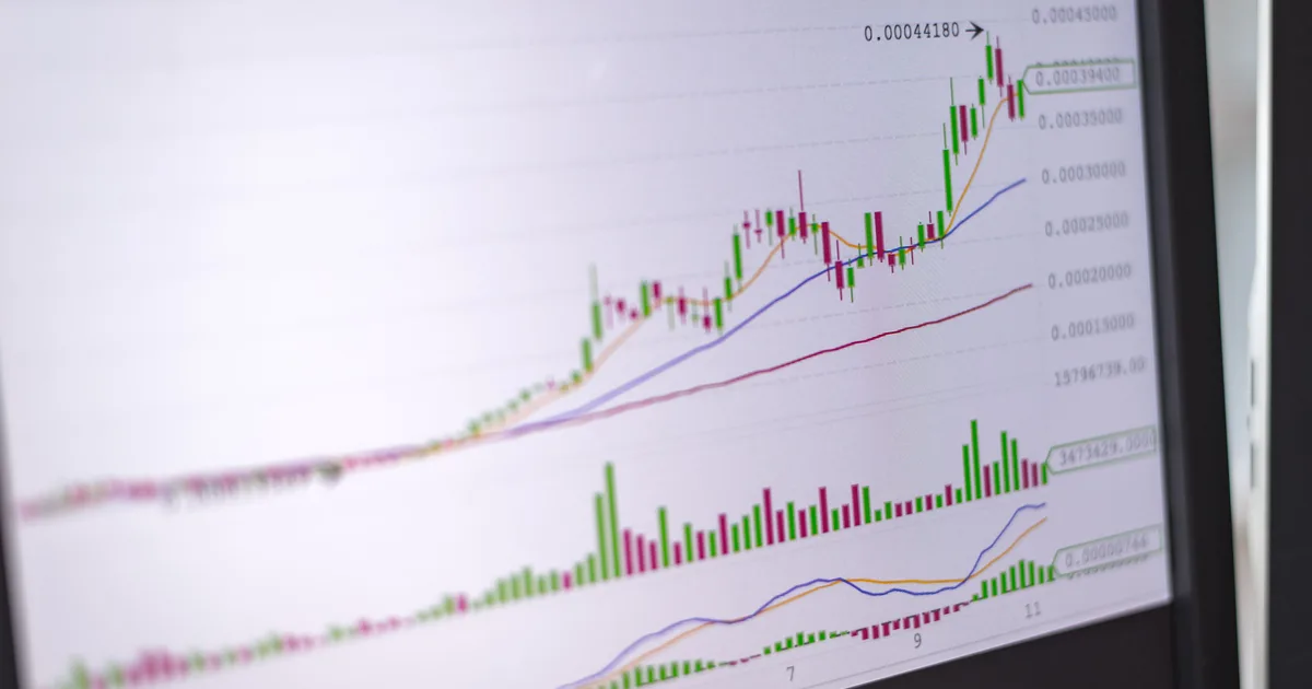
A convolutional neural network for the stock market slides small learned filters across a window of recent prices and volume, and learns which local shapes tend to come before an up move or a down move. It can find real signal. The best published result, a 2023 Journal of Finance study that fed a CNN black-and-white price charts, beat classic momentum and reversal strategies across 19 years of US data the model had never seen. The same study shows where that edge lives: in heavy weekly trading, mostly in smaller stocks, with returns that shrink once costs and size limits apply.

One note before the code. Nothing here is investment advice, and a backtest is a claim about the past. Treat any model you build as a research project until it has survived data it was never tuned on.

How a convolutional neural network reads stock prices

A CNN looks for small patterns wherever they appear. In photos that means edges and corners. In a price series it means short shapes, such as three falling days followed by a spike in volume.

The mechanism is the convolution. A filter, meaning a short list of learned weights, slides along the input and produces a high value wherever the local data matches its shape. Stacking layers lets early filters catch two-day wiggles while later ones combine them into week-long patterns. Pooling layers keep the strongest match in each stretch, so the network cares that a pattern happened and cares less about which Tuesday.

There are two common ways to feed it market data. The first treats the series as a one-dimensional signal: each sample is a window of days, and each input channel is one feature such as daily return. The second draws the window as a picture. Jiang, Kelly and Xiu render each stock's recent price bars and trading volume as a black-and-white image, three pixels wide per day, and train a two-dimensional CNN on the charts.

Technical analysts have stared at charts for a century. This is the first chartist that can be retrained overnight and never claims afterwards that it saw the move coming.

How to determine input layers for a neural network on price data

The input layer's shape is the number of features by the number of days in the window. Picking those two numbers is most of the modelling work.

Start with the window length. Jiang, Kelly and Xiu tested windows from 5 to 60 trading days, roughly a week up to a quarter. Longer windows give the filters more context and leave fewer independent samples per stock.

Then choose the channels. Raw prices make a poor input, because a network trained on a stock at $50 has no idea what to do with the same stock at $200. Use returns, and scale volume against its own recent average. Each feature becomes one channel, so returns plus volume gives an input of 2 by 20. Some teams add a news-sentiment channel built with natural language processing in finance.

The label needs the most care. A common setup asks a yes-or-no question: did the stock rise over the next five days? That turns forecasting into classification, and the output layer becomes a single number squeezed into a probability.

The most expensive bug in this field is lookahead, meaning a feature that quietly contains information from after the prediction date. Scaling volume by its average over the whole dataset does it. Shuffling samples before the train and test split does it too, because overlapping windows let the model memorise answers it will later be tested on. Split by date, and leave a gap of one forecast horizon between the training and test data.

A PyTorch neural network in Python for stock direction

Here is a small one-dimensional CNN in PyTorch. It builds samples from arrays of closing prices and volumes, then trains a classifier that outputs the probability of an up move over the next five days.

import numpy as np
import torch
from torch import nn

def make_samples(close, volume, window=20, horizon=5):
    ret = np.diff(np.log(close))              # daily log returns
    vol = volume[1:]
    X, y = [], []
    for t in range(window, len(ret) - horizon + 1):
        v = vol[t - window:t]
        X.append([ret[t - window:t], np.log(v / v.mean())])  # 2 channels
        y.append(float(ret[t:t + horizon].sum() > 0))         # up in 5 days?
    return torch.tensor(np.array(X), dtype=torch.float32), torch.tensor(y)

model = nn.Sequential(
    nn.Conv1d(2, 16, kernel_size=5, padding=2), nn.ReLU(),
    nn.MaxPool1d(2),
    nn.Conv1d(16, 32, kernel_size=5, padding=2), nn.ReLU(),
    nn.AdaptiveMaxPool1d(1), nn.Flatten(),
    nn.Linear(32, 1),                         # one logit for "up"
)

X, y = make_samples(close, volume)
cut = int(len(X) * 0.7)                       # split by time, never shuffle
X_train, y_train = X[:cut], y[:cut]
X_test, y_test = X[cut + 5:], y[cut + 5:]     # gap of one horizon

loss_fn = nn.BCEWithLogitsLoss()
opt = torch.optim.Adam(model.parameters(), lr=3e-4)
for epoch in range(200):
    loss = loss_fn(model(X_train).squeeze(1), y_train)
    opt.zero_grad()
    loss.backward()
    opt.step()

The tensor shape matches what the PyTorch Conv1d layer expects, with the batch first and the sequence length last. A kernel of 5 with padding of 2 keeps the length at 20, and pooling halves it to 10. The adaptive pool then collapses what is left to the strongest response per filter.

Run it on random-walk prices first. Test accuracy should hover around 50%, and that is the correct result. A pipeline that beats a coin flip on coin flips has found a bug, and bugs rarely compound at 20% a year.

Accuracy is a weak score here anyway. A model can be right 51% of the time and still lose money if its misses land on the big days, so read the full classification report for the model and then judge it on returns. If the training loss refuses to move, the debugging order in our neural network recipes guide applies unchanged.

Trader reviewing price charts on several monitors, the kind of data a convolutional neural network for the stock market learns from — Photo by AlphaTradeZone on Pexels

What CNN stock market research actually found

The strongest evidence comes from Jiang, Kelly and Xiu's chart-image study. They trained once on US stocks from 1993 to 2000, then held the model fixed for a test period running from 2001 to 2019.

Each week they sorted stocks by the CNN's predicted probability. The strategy bought the top tenth and shorted the bottom tenth. With equal weights, that earned an annualised gross Sharpe ratio as high as 7.2. A Sharpe ratio measures return per unit of risk, and anything above 1 over a long test is respectable. With value weights, where big companies count for more, the figure fell to 1.7. The closest classic rivals reached equal-weight Sharpe ratios of 2.9 and 2.8.

The fine print matters as much as the headline. The weekly strategy ran monthly turnover near 690%, which the authors say suits market makers more than ordinary investors. After standard trading costs the best weekly figure fell to 4.0, and restricted to the 500 largest stocks the Sharpe ratios stayed above 1. The learned patterns also travelled: a model trained on US stocks worked in international markets.

Explainable AI in finance usually means showing which inputs drove a forecast, and a CNN makes that hard. The authors probed what their model favoured and found patterns that differ significantly from the trend signals analysts usually test, which is part of why the result persuaded people.

Other work points the same way with smaller claims. CNNpred, from Hoseinzade and Haratizadeh, predicts next-day direction for major US indices such as the S&P 500, and gets its edge by feeding the network data from several markets at once. Plenty of papers in this space test one index over one period, the research equivalent of a fund brochure that only lists its good years.

Overcoming catastrophic forgetting in neural networks when markets change

Markets change their behaviour, usually right after you finish tuning. Retraining fixes the drift, with a catch.

Catastrophic forgetting is what happens when a network trained on new data overwrites what it learned from old data. In markets you want some of that, since patterns from 2009 may be useless today. You also want the model to remember rare events such as crashes, which show up perhaps once a decade.

The standard answer is walk-forward training. Retrain on a rolling window, then test only on the period that follows. Repeat as the window moves forward. Keeping a sample of older stress periods in every training set, a technique called replay, protects the rare cases. Jiang, Kelly and Xiu trained once to save compute and note that rolling retraining would likely improve their predictions.

Every retrain is also another chance to overfit. Each architecture or window you try against the same test period raises the odds that the winner is luck. Keep a final stretch of data you touch once, at the end, and write down how many variants you tried before you looked.

A checklist before you trust the backtest

Inputs are returns and relative volume, never raw prices.
Training and test data are split by date, with a gap of one forecast horizon.
Random-walk data scores close to 50%.
Results are reported after trading costs, on stocks you could trade in size.
A final holdout period exists and has been touched once.

Pass all five and you have a research result worth a second look. For the training and evaluation habits underneath it, LLM Systems Engineering covers data budgets and model evaluation in depth, even though its subject is language models.

Convolutional Neural Network Stock Market Prediction: What Works